Neural Radiance Fields from Scratch

Neural Radiance Fields (NeRFs) were one of the first models that made neural rendering actually work. They map from 3D coordinates and view directions to density and color, and when trained on enough posed images, they produce photorealistic novel views of a scene.

I implemented the core NeRF pipeline from scratch in PyTorch based on the original NeRF paper. Below I'll walk through the main components I built, with references back to the original paper, including equations and images where relevant.

Background

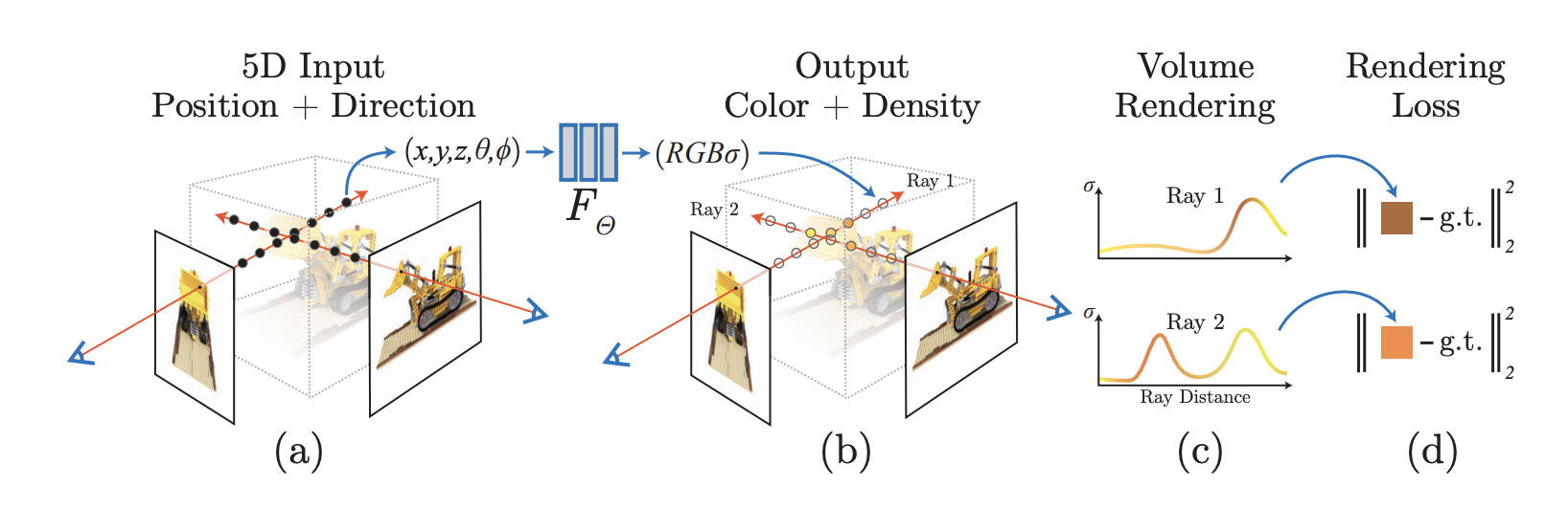
NeRF concept overview

Neural Radiance Fields (NeRF) represent a scene as a continuous volumetric field and use a neural network to map a 3D point and a viewing direction to a colour and opacity. The method implicitly parameterises a scene with a multi-layer perceptron (MLP) that takes a 3D position x and a view direction d and outputs a colour vector c and a density value σ. The colour integrates emitted radiance along the ray and the density acts like a probability of encountering matter along the ray. Rendering novel views becomes an instance of numerical quadrature: the continuous rendering integral

C(r)=\int_{\mathrm{near}}^{\mathrm{far}}T(z)\,\sigma(z)\,c(z,\mathbf{d})\,\mathrm{d}z\;\text{with}\;T(z)=\exp\Bigl(-\int_{\mathrm{near}}^{z}\sigma(s)\,\mathrm{d}s\Bigr)

is approximated with a discrete sum of sampled points along each ray. Through numerical quadrature the NeRF renderer computes the expectation of emitted radiance

\hat{C}(r)=\sum_{i=1}^{N}T_i\bigl(1-e^{-\sigma_i\delta_i}\bigr)c_i\,,\quad T_i=\exp\Bigl(-\sum_{j=1}^{i-1}\sigma_j\delta_j\Bigr)

which resembles the familiar alpha-compositing formula in computer graphics. Below is a walkthrough of our implementation for the COS 526 assignment.

Part 1 — Network architecture

NeRF network architecture diagram, from original NeRF paper

The NeRF MLP accepts a positional encoding of the 3D point and, optionally, a positional encoding of the view direction. Following the original architecture, the network contains D fully connected layers of width W with ReLU activations. A skip connection is introduced at layer 4: the encoded position (dimension 60) is concatenated with the activations of layer 4 and fed into layer 5, helping the network "remember" positional information. After eight layers the scalar volume density σ is produced and a ReLU is applied to enforce non-negativity. The view-dependent branch then concatenates the encoded viewing direction (dimension 24) with the features from the previous layer and outputs a 3-element colour vector. Concretely, our PyTorch implementation defines a list of linear layers for the position branch and separate linear layers for the feature, density and RGB heads:

class NeRFNetwork(nn.Module):
    def __init__(self, input_ch, input_ch_dir, W=256, D=8, skips=[4], use_viewdirs=True):
        super().__init__()
        # D fully connected layers with optional skip connections
        self.pts_linears = nn.ModuleList([
            nn.Linear(input_ch, W)
        ] + [
            nn.Linear(W + input_ch, W) if i in skips else nn.Linear(W, W)
            for i in range(1, D)
        ])
        # feature and head layers
        self.feature_linear = nn.Linear(W, W)
        self.alpha_linear   = nn.Linear(W, 1)  # density σ
        self.rgb_linear     = nn.Linear(W // 2, 3)  # RGB colour
        self.use_viewdirs   = use_viewdirs

    def forward(self, x, d):
        h = x
        for i, layer in enumerate(self.pts_linears):
            h = F.relu(layer(h))
            # inject the encoded position at the skip layer
            if i in self.skips:
                h = torch.cat([x, h], dim=-1)
        sigma = F.relu(self.alpha_linear(h))  # non-negative density
        feature = self.feature_linear(h)
        if self.use_viewdirs:
            h = torch.cat([feature, d], dim=-1)
        rgb = torch.sigmoid(self.rgb_linear(h))
        return rgb, sigma

Part 2 — Raw density to alpha conversion

After the network predicts a raw density σ for each sampled point along a ray, the values must be transformed into alpha opacities. Following the discretised volume-rendering equation, we compute

\alpha_i = 1 - \exp(-\max(\sigma_i,0)\,\delta_i)

where δᵢ is the distance between adjacent samples. The ReLU activation ensures non-negative density values, and the exponential translates density to a probability of opacity. In code this is a single-line transformation:

alpha = 1.0 - torch.exp(-F.relu(raw_sigma) * dists)

Part 3 — Volumetric rendering

To render a pixel, we accumulate contributions from all sample points along the ray using the transmittance weights. We first compute the cumulative transmittance Tᵢ=∏ⱼ<ᵢ(1-αⱼ), then the weight of the i-th sample is wᵢ = αᵢTᵢ. These weights sum to the accumulated opacity and act as mixing coefficients for colour and depth. Given the per-sample colour vectors c and depths z, the final outputs are

transparency = 1.0 - alpha
cumulative_transmittance = torch.cumprod(torch.cat([torch.ones_like(alpha[..., :1]), transparency], dim=-1), dim=-1)
transmittance = cumulative_transmittance[..., :-1]
weights = alpha * transmittance
rgb_map   = torch.sum(weights[..., None] * rgb, dim=-2)      # weighted colour
depth_map = torch.sum(weights * z_vals, dim=-1)               # expected depth
disp_map  = 1.0 / torch.clamp(depth_map / torch.sum(weights, -1), min=1e-10)
acc_map   = torch.sum(weights, -1)                            # accumulated opacity

This procedure directly implements the discretised rendering equation in a way that is fully differentiable.

Part 4 — Point sampling along rays

For each ray we sample N points between the near and far clipping planes. Given a ray origin o and direction d, and an array of depths z₁,...,zₙ, the world-space coordinates are

pts = rays_o[..., None, :] + rays_d[..., None, :] * z_vals[..., :, None]

Broadcasting over rays and samples yields a tensor of shape (n_rays, n_samples, 3). These points are passed through the positional encoding before being fed into the network.

Part 5 — Positional encoding

High-frequency functions are difficult for ReLU networks to approximate. The NeRF authors therefore apply a sinusoidal positional encoding to each coordinate, effectively embedding a 3D vector into a higher-dimensional space using sine and cosine functions at multiple frequencies. Frequencies can be linearly or logarithmically spaced. For log-sampling we use 2ᵏ for k∈[0,max_freq]; for linear sampling we use evenly spaced frequencies between 2⁰ and 2^max_freq. The embedding produces features that retain both low-frequency structure and fine details. In code the embedding is built by iterating over each frequency and applying sine and cosine:

if log_sampling:
    freq_bands = 2.0 ** torch.linspace(0.0, max_freq, N_freqs)
else:
    freq_bands = torch.linspace(2.0 ** 0.0, 2.0 ** max_freq, N_freqs)
embed_fns = [lambda x: x]  # include the identity if desired
for freq in freq_bands:
    embed_fns.append(lambda x, freq=freq: torch.sin(x * freq))
    embed_fns.append(lambda x, freq=freq: torch.cos(x * freq))

This yields a feature vector of dimension 2×N_freqs×input_dims, which is concatenated with the identity if required. The network then operates on these encoded inputs.

Representative renderings

Training a NeRF requires tens of thousands of gradient steps. Below are representative outputs from our implementation on two LLFF scenes—lego and fern—at increasing iteration counts. Early iterations produce blurry images; as training proceeds the model learns geometry and lighting, producing sharper details and more accurate shadows.

Lego scene

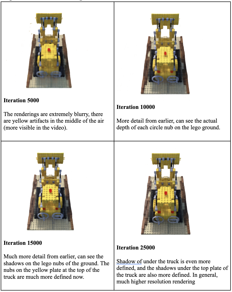
NeRF training progression on LEGO scene

The LEGO truck scene shows four snapshots at 5,000, 10,000, 15,000 and 25,000 training iterations. Early on the model only captures coarse shapes—renderings are extremely blurry and yellow artefacts float in mid-air. By 10,000 iterations the network has learned enough structure to reveal the circular nubs on the ground, though edges are still soft. At 15,000 iterations the shadows cast by the LEGO nubs on the ground and the nubs on the top plate become more pronounced. By 25,000 iterations the shadows beneath the truck and under its roof are well resolved and the reconstruction appears crisp and high resolution.

Fern scene

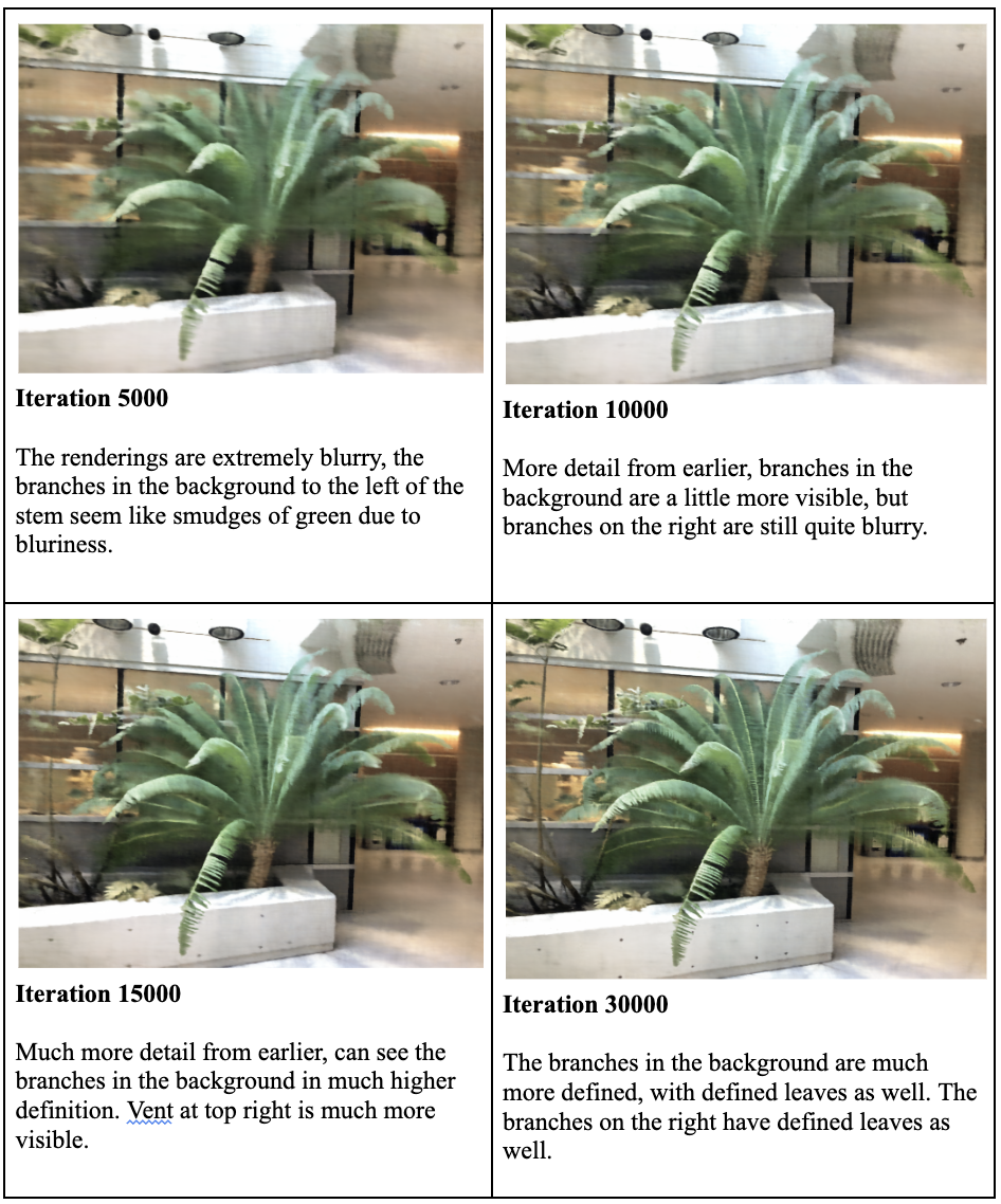
NeRF training progression on Fern scene

The fern scene exhibits a similar progression. At 5,000 iterations the reconstruction is extremely blurry—the fronds appear as smudges and the background branches are indistinguishable. After 10,000 iterations the left-hand leaves and some background branches become discernible, but the right-hand fronds are still blurred. At 15,000 iterations the network resolves the leaves and background details, and even the vent near the top of the scene becomes visible. By 30,000 iterations the fern's leaves are fully defined across the entire scene with accurate shadows and highlights, demonstrating the power of the model to capture fine textures and lighting.

Results and Discussion

The NeRF pipeline we implemented follows the reference architecture closely. Skip connections allow deeper layers to retain positional information, and separating density and colour predictions ensures that the density depends only on position. The raw density-to-alpha conversion and volumetric rendering operations implement the discrete version of the rendering integral, yielding differentiable outputs for end-to-end training. Positional encoding injects high-frequency signals, enabling the MLP to capture fine details.

During training we observed that the quality of the renderings improves steadily with more iterations. Early images capture coarse structure but are dominated by blurriness and artefacts. As the network learns, both geometry (depth and shape) and radiance (colour and shading) become more accurate. After around 25-30k iterations the model produces sharp results with realistic shadows and fine textures. Further improvements could come from hierarchical sampling—using separate coarse and fine networks to allocate more samples near high-density regions—or from recent advances such as Instant NeRF for faster training.