Deep Convolutional GAN from Scratch

GANs (Generative Adversarial Networks) pit two networks against each other: a generator that synthesizes images from random noise, and a discriminator that tries to tell apart real images from fakes. Through this adversarial training, the generator gradually learns to create outputs indistinguishable from the dataset.

I implemented a Deep Convolutional GAN (DCGAN) from scratch in PyTorch, training it on Fashion-MNIST. Below I'll walk through the architecture, training loop, and key implementation details, along with results from different stages of training.

Generator Architecture

The generator follows the standard DCGAN design: it takes a 100-dimensional noise vector and progressively upsamples it through transposed convolutions into a

32 \times 32

image. The key insight is that by stacking deconvolutional layers with batch normalization, we can generate high-quality images from pure noise.

class DCGenerator(nn.Module):
    def __init__(self, noise_size=100, conv_dim=64, spectral_norm=False, is_col=False):
        super(DCGenerator, self).__init__()
        self.final_output = 3 if is_col else 1
        
        # Initial projection from noise to feature maps
        self.linear_bn = nn.Sequential(
            nn.ConvTranspose2d(noise_size, conv_dim * 4, 4, 1, 0, bias=False),
            nn.BatchNorm2d(conv_dim * 4)
        )
        
        # Progressive upsampling layers
        self.upconv1 = self._upconv_block(conv_dim * 4, conv_dim * 2, 3, 2, 1)
        self.upconv2 = self._upconv_block(conv_dim * 2, conv_dim, 3, 2, 1)
        self.upconv3 = nn.ConvTranspose2d(conv_dim, self.final_output, 4, 2, 1, bias=False)

    def _upconv_block(self, in_channels, out_channels, kernel_size, stride, padding):
        """Helper function to create upconv block with batch norm"""
        return nn.Sequential(
            nn.ConvTranspose2d(in_channels, out_channels, kernel_size, stride, padding, bias=False),
            nn.BatchNorm2d(out_channels)
        )

    def forward(self, z):
        # z shape: (batch_size, noise_size, 1, 1)
        out = F.relu(self.linear_bn(z))  # (batch_size, 256, 4, 4)
        out = F.relu(self.upconv1(out))  # (batch_size, 128, 8, 8)
        out = F.relu(self.upconv2(out))  # (batch_size, 64, 16, 16)
        out = torch.tanh(self.upconv3(out))  # (batch_size, 1, 32, 32)
        return out

The architecture follows several key design principles. The input consists of

z \sim \mathcal{U}(-1,1)^{100}

— uniform noise in 100 dimensions. Each layer progressively doubles the spatial resolution through upsampling. Batch normalization is applied after each transposed convolution except the output layer. For activations, ReLU is used in hidden layers while

\tanh

is used for the output to map values to the [-1,1] range. Following DCGAN best practices, no bias terms are used when batch normalization is present.

The noise vector is first projected to a

4 \times 4

feature map with 256 channels, then progressively upsampled to

32 \times 32

with decreasing channel count. This creates a classic "inverted pyramid" structure that's effective for image generation.

Discriminator Architecture

The discriminator mirrors the generator, progressively downsampling

32 \times 32

images into a single scalar representing the probability that the input is real. It uses strided convolutions instead of pooling to maintain gradient flow throughout the network.

class DCDiscriminator(nn.Module):
    def __init__(self, conv_dim=64, spectral_norm=False, is_col=False):
        super(DCDiscriminator, self).__init__()
        self.input_channel = 3 if is_col else 1
        
        # Progressive downsampling layers
        self.conv1 = self._conv_block(self.input_channel, conv_dim, 5, 2, batch_norm=False)
        self.conv2 = self._conv_block(conv_dim, conv_dim * 2, 5, 2)
        self.conv3 = self._conv_block(conv_dim * 2, conv_dim * 4, 5, 2)
        self.conv4 = nn.Conv2d(conv_dim * 4, 1, 5, 2, padding=1, bias=True)
        
        # Optional spectral normalization for training stability
        if spectral_norm:
            self.conv1 = nn.utils.spectral_norm(self.conv1)
            self.conv2 = nn.utils.spectral_norm(self.conv2)
            self.conv3 = nn.utils.spectral_norm(self.conv3)
            self.conv4 = nn.utils.spectral_norm(self.conv4)

    def _conv_block(self, in_channels, out_channels, kernel_size, stride, batch_norm=True):
        """Helper function to create conv block with optional batch norm"""
        layers = [nn.Conv2d(in_channels, out_channels, kernel_size, stride, 
                           padding=kernel_size//2, bias=not batch_norm)]
        if batch_norm:
            layers.append(nn.BatchNorm2d(out_channels))
        return nn.Sequential(*layers)

    def forward(self, x):
        # x shape: (batch_size, 1, 32, 32)
        out = F.leaky_relu(self.conv1(x), negative_slope=0.2)  # (batch_size, 64, 16, 16)
        out = F.leaky_relu(self.conv2(out), negative_slope=0.2)  # (batch_size, 128, 8, 8)
        out = F.leaky_relu(self.conv3(out), negative_slope=0.2)  # (batch_size, 256, 4, 4)
        out = self.conv4(out).squeeze()  # (batch_size, 1) -> (batch_size,)
        return out

Several key design choices define the discriminator architecture. Strided convolutions replace pooling operations to allow the network to learn its own downsampling. LeakyReLU activations with a negative slope of 0.2 prevent dying neurons, which can be problematic with standard ReLU. The first layer excludes batch normalization to allow the network to learn input-dependent features directly from raw pixel values. Optional spectral normalization constrains the Lipschitz constant for improved training stability. The progressive channel doubling increases representational capacity as spatial dimensions decrease.

The discriminator takes a

32 \times 32

image and reduces it to a single scalar through four convolutional layers, halving the spatial dimensions at each step while doubling the channel count.

Training Loop and Loss Functions

Instead of the standard GAN loss, I implemented the Wasserstein GAN (WGAN) objective, which provides more stable training and meaningful loss curves. The WGAN loss approximates the Earth-Mover distance between real and generated distributions.

Wasserstein Loss Implementation

The WGAN objective is:

\min_G \max_{D \in \mathcal{D}} \mathbb{E}_{x \sim p_r}[D(x)] - \mathbb{E}_{z \sim p_z}[D(G(z))]

where

\mathcal{D}

is the set of 1-Lipschitz functions. In practice, I enforce the Lipschitz constraint through spectral normalization rather than weight clipping.

def train_step(real_images, generator, discriminator, g_optimizer, d_optimizer, opts):
    batch_size = real_images.size(0)
    real_images = real_images.to(opts.device)
    
    # Train Discriminator (Critic) - maximize D(real) - D(fake)
    d_optimizer.zero_grad()
    
    # Real images - want to maximize D(real)
    d_real_output = discriminator(real_images)
    d_real_loss = -torch.mean(d_real_output)
    
    # Fake images - want to minimize D(fake)
    noise = sample_noise(batch_size, opts.noise_size, opts.device)
    fake_images = generator(noise)
    d_fake_output = discriminator(fake_images.detach())  # detach to avoid generator gradients
    d_fake_loss = torch.mean(d_fake_output)
    
    # Total discriminator loss
    d_total_loss = d_real_loss + d_fake_loss
    d_total_loss.backward()
    d_optimizer.step()
    
    # Train Generator - maximize D(G(z))
    g_optimizer.zero_grad()
    noise = sample_noise(batch_size, opts.noise_size, opts.device)
    fake_images = generator(noise)
    g_output = discriminator(fake_images)
    g_loss = -torch.mean(g_output)  # want to maximize D(fake)
    g_loss.backward()
    g_optimizer.step()
    
    return d_total_loss.item(), g_loss.item()

def sample_noise(batch_size, noise_size, device):
    """Sample random noise from uniform distribution [-1, 1]"""
    return torch.rand(batch_size, noise_size, 1, 1, device=device) * 2 - 1

Training Configuration

I found that careful hyperparameter tuning was crucial for stable training:

# Optimizer settings - asymmetric learning rates
generator_lr = 3e-5
discriminator_lr = 6e-5  # Discriminator learns faster

g_optimizer = torch.optim.Adam(generator.parameters(), 
                               lr=generator_lr, 
                               betas=(0.5, 0.999))
d_optimizer = torch.optim.Adam(discriminator.parameters(), 
                               lr=discriminator_lr, 
                               betas=(0.5, 0.999))

# Training parameters
batch_size = 32
train_iters = 20000
noise_size = 100

Training Results and Evolution

The progression of generated images during training reveals how the generator gradually learns the underlying data distribution. Below is the training progression across 20,000 iterations:

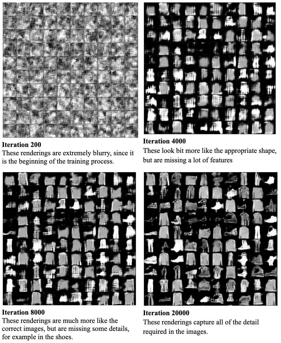
DCGAN training progression on Fashion-MNIST

Training Stage Analysis

Iteration 200 (Early Training): At this stage, the generator produces essentially random noise with slight spatial correlation. The discriminator has learned to reject these obviously fake images, but the generator hasn't learned meaningful features yet. We see extremely blurry, blob-like shapes with no recognizable structure.

Iteration 4000 (Feature Emergence): Clothing outlines begin to emerge as the generator learns basic spatial relationships. The discriminator is forcing the generator to produce images with the right overall intensity distribution, but fine details are still completely missing. We can start to distinguish between different garment types, though they're heavily blurred.

Iteration 8000 (Shape Refinement): Generated images now clearly resemble Fashion-MNIST items. The generator has learned the general shapes and proportions of clothes, shoes, and accessories. However, fine details like textures, patterns, and sharp edges are still fuzzy. The discriminator is now sophisticated enough to reject images without proper shape consistency.

Iteration 20000 (Detail Convergence): The final stage shows impressive results: sharp edges, diverse clothing types, and realistic textures. The generator has learned to capture most of the dataset's variation, producing images that are difficult to distinguish from real Fashion-MNIST samples. Notice how shoes now have clear soles, shirts have defined necklines, and bags have handles and structure.

Learnings

The most crucial finding was that discriminator must learn faster than the generator. When

lr_G \geq lr_D

, the generator would collapse to a single mode, producing identical outputs regardless of input noise. The sweet spot was

lr_D = 6 \times 10^{-5}

and

lr_G = 3 \times 10^{-5}

. This asymmetry ensures the discriminator stays ahead, providing meaningful gradients to the generator.

This DCGAN implementation demonstrates both the power and fragility of adversarial training. Even on Fashion-MNIST, a relatively simple grayscale dataset, achieving stable training required careful hyperparameter tuning and architectural choices. However, when properly configured, the model produces sharp, diverse images of clothing from pure noise.

The key takeaways from this implementation are significant. Wasserstein loss provides more stable training than vanilla GAN loss, eliminating many of the convergence issues associated with the original formulation. Asymmetric learning rates with

lr_D > lr_G

are crucial for avoiding generator collapse and maintaining training stability. Spectral normalization proves to be an effective and computationally efficient regularization technique that constrains the discriminator's Lipschitz constant. Finally, batch size significantly impacts training dynamics, with larger batches generally providing more stable convergence.

The natural next step would be scaling this implementation to more complex datasets like CIFAR-10 or CelebA, where techniques like progressive growing, self-attention, and more sophisticated regularization become necessary. Additionally, exploring more recent GAN variants like StyleGAN or implementing unconditional generation would be valuable extensions.